Hypothesis Testing
Prueba de hipótesis
Recibido: 28-03-2022
Aceptado: 29-03-2022
Publicado: 31-03-2022
Revista MetroCiencia
Volumen 30, Número 1, 2022
Editorial Hospital Metropolitano
Isaac Zhao1, María Carolina Velasco2
The present paper is a practical guide on hypothesis testing. It covers various statistical inference methods that are widely applied in research studies. To avoid narrowing down statistical problems to p-values, we discuss common misuses and misinterpretations of statistical tests and emphasize the importance of interpreting results in the context of the study design, previous knowledge, and complementary analyses. We provide a toolkit that reinforces good scientific practice.
Keywords: hypothesis testing, p-value, statistical significance, z-test, t-test, ANOVA, chi-squared, f-test, correlation coefficient.
Este artículo es una guía práctica sobre la prueba de hipótesis. Cubre varios métodos de inferencia estadística utilizados extensamente en estudios de investigación para evaluar supuestos. Con el objetivo de evitar reducir problemas estadísticos a los valores p, discutimos aplicaciones e interpretaciones erróneas de las pruebas estadísticas y enfatizamos la importancia de interpretar los resultados en el contexto del diseño del estudio, el conocimiento previo y los análisis complementarios. Así, el artículo proporciona herramientas que promueven el uso de buenas prácticas científicas.
Palabras clave: prueba de hipótesis, valor p, significancia estadística, prueba z, prueba t, ANOVA, chi-cuadrado, prueba F, coeficiente de correlación.
Isaac Zhao
![]() https://orcid.org/0000-0002-4352-4969
https://orcid.org/0000-0002-4352-4969
María Carolina Velasco
![]() https://orcid.org/0000-0002-8482-9865
https://orcid.org/0000-0002-8482-9865
 |
Este artículo está bajo una licencia de Creative Commons de tipo Reconocimiento – No comercial – Sin obras derivadas 4.0 International. |
*Correspondencia: ma.carolina.velasco@gmail.com
Hypothesis testing evaluates research claims or assumptions about population characteristics given observed data. Based on the scientific method, it provides a standardized process for researchers to perform statistical analyses that evaluate the strength of evidence for a question of interest. However, statistical significance in hypothesis testing can be often misunderstood and misused in the research community. Much of the blame is placed on traditional statistical training and textbooks that reduce statistical problems to p-values. The present paper aims to provide a critical and practical guide on hypothesis testing methods by drawing from Shahbaba’s introductory book to biostatistics using R10, the American Statistical Association’s (ASA) statement on p-values11, and Greenland et al.’s guide to misinterpretations of statistical tests, p-values, confidence intervals, and power6.
2.1 Formulate the Null and Alternative Hypotheses
Hypothesis testing provides researchers with a testable framework to assess statements about their scientific question. However, each framework relies on various assumptions about how the data was collected and analyzed, and how the results were interpreted and reported. These assumptions are embodied in all statistical models, which, in turn, support statistical methods. As noted by Greenland et al. and Wassertain et al., there are important considerations that researchers must take into account when building statistical models6,11. First, although a model is supposed to represent the data variability, the assumptions used to build it are not always realistic or justified. Second, the model might not have the adequate scope to represent both the observed and hypothetical alternative data. Third, the model might be too abstract or not represented at all in a study, leading researchers and readers to overlook assumptions6,11.
Despite these limitations, assumptions underpin all statistical methods and interpretations. A key assumption in statistical testing is the definition of the null and alternative hypotheses. The null hypothesis (denoted H0) of a study is a statement about a non-existing association between the measured variables. H0 states that the population parameter is equal to a prespecified value such as 0, or that two population parameters are equal.
Contrary to the null hypothesis, the alternative hypothesis (denoted HA) is a statement about an existing relationship between the measured variables. HA can be written as a one-sided or two sided comparison. A one-sided HA is unidirectional and describes the case when the population parameter of interest is greater or lower than a prespecified value or another population parameter. A two-sided HA is bi-directional and describes the case when the population parameter of interest is not equal to a prespecified value or to another population parameter.
2.2 Set the Significance Level
The significance level, α, is a pre-specified probability threshold below which researchers can reject the null hypothesis. The most common value of α is 0.05. However, depending on the scope and aim of the study, different levels of significance may be set such as 0.1 and 0.01. The significance level represents the probability we place on a test for incorrectly rejecting H0, which is called the type I error of the test10.
Readers should not confuse the significance level with the p-value6. The significance level is a cut-off value set prior to the statistical test. The p-value is often referred to as the “observed significance level” because it is used to assess whether results are significant or not assuming H0 to be true. Refer to Section 2.4 that provides a discussion about p-values.
2.3 Perform the Appropriate Statistical Test
The choice of running a particular hypothesis test depends on the type of data collected. We can run univariate and multivariate tests for continuous and/or categorical variables. Many of these tests are covered in Sections 3 and 4.
The type of test determines the test statistic. The test statistic is a summary measure computed from the sample data to quantify the distance between the observed data and the predicted model under H06. This measure is a random variable, meaning that we may get different estimates each time we take a different sample from the population. If the null hypothesis is indeed true, we would expect the values to be close to the known distribution of H0, and vice versa10. In reality, we have only one estimate for the test statistic and the further it is from the value stated by H0, the stronger the evidence is against it.
2.4 Determine Statistical Significance and Reach Conclusions
A measure that is widely (and often inadequately) reported alongside the test statistic is the p-value. As defined by Greenland et al., the p-value is the probability that the chosen test statistic would have been at least as large as its observed value if every model assumption were correct, including H06. In broader terms, the p-value measures the fit of the model to the observed data6,11.
It is important to note that the p-value is not the probability that the null hypothesis is true6,11. In fact, the p-value already assumes H0 to be the truth. Therefore, if all the model assumptions are correct, a p-value that is smaller than the significance level, say α=0.05, suggests that the data does not support H0. In such a case, the null hypothesis is rejected and the result is deemed “statistically significant”. In contrast, a p-value that is larger than α suggests that the observed data was generated according to the null. Hence, the null is not rejected and the result is deemed “nonsignificant”. Failing to reject H0 simply means that the results are inconclusive rather than implying that the null hypothesis is true10.
A fundamental disclaimer when discussing p-values is that statistically significant results may not be reproducible or replicable. Large random errors or violated assumptions may lead to unreliable p-values and, hence, invalid claims6. This is why the p-value should not be the only means by which we evaluate research questions. Instead, as the American Statistical Association recommends, we must also consider prior knowledge, the design of the study, the validity of the model assumptions, and the quality of the measurements11. Only then can we claim scientific findings that inform business and policy decisions.
After covering the basic concepts and steps required to conduct hypothesis testing, we present a practical guide to run tests for one or various population parameters in R8. The significance level set for all the tests is α=0.05. To exemplify the tests, we analyze the dataset called “Survival from Malignant Melanoma” (referred to as melanoma moving forward). The dataset, publicly available in the “boot” package in R, contains demographic and tumor characteristics of patients with malignant melanoma in Denmark¹.
3.1 One Population Mean
The one-sample t-test is used to test if the population mean of a continuous variable is significantly different than a hypothesized value, assuming that the population variance is unknown. This test uses the t-statistic, which is comparable to the z-statistic (also called z-score) when the sample size is large or the population variance is known.
The primary assumptions of the t-test are the following7:
A melanoma tumor thickness greater than 4 mm is associated with a higher chance of treatment recurrence2. To test if the population mean of tumor thickness (denoted as µ) is greater than 4 mm in the melanoma study, we set a one-sided alternative hypothesis. Accordingly, the null and alternative hypotheses are:
H0: µ ≤ 4. The population mean tumor thickness is less than or equal to 4 mm.
HA: µ > 4. The population mean tumor thickness is greater than 4 mm.
We then run a one-sided, one-sample t-test with the R code shown below. By default, the t.test function assumes a hypothesized mean of 0, computes a two-tailed hypothesis test, and estimates the 95% confidence interval for the population mean. The arguments mu (hypothesized population mean), alternative (one or two sided HA), and conf.level (confidence level of interval) can be easily modified as shown in the code below.
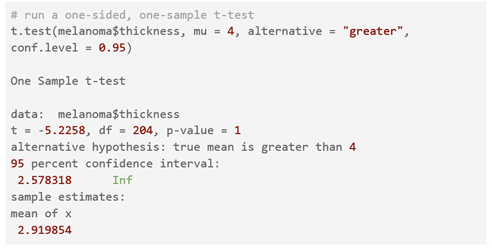
The sample mean of tumor thickness is 2.9 millimeters and the one-sided t-test computes a p-value of 1. Since the p-value is greater than the significance level of α=0.05, we fail to reject the null hypothesis and cannot conclude that the mean tumor thickness is greater than 4. This is corroborated by the 95% confidence interval; it suggests that we are 95% confident that the true population mean is greater than or equal to 2.58, which includes the hypothesized value of 4.
3.2 One Population Proportion
The one-sample proportion test evaluates if the population proportion of a group from a categorical variable is significantly different than a given value. For binary variables, the population proportion is the same as the population mean. Therefore, we can run a z-test in which the test statistic is the z-score.
The assumptions for a proportion test are the following4:
H0: p = 0.5. The population proportion of males in our study is 0.5.
HA: p ≠ 0.5. The population proportion of males in our study is not 0.5.
We then run a two-sided, one-sample proportion test with the R code shown below. By default, the prop.test function assumes a hypothesized proportion of 0.5, computes a two-tailed hypothesis test, and estimates the 95% confidence interval for the population proportion. The arguments x (the number of observations of the grouping of interest), n (total number of observations), p (the hypothesized proportion of the grouping of interest), alternative (one or two sided Ha), and conf.level (confidence level of the interval) can be easily modified as shown in the code.

The sample proportion of males is 39% and the two-sided, one-sample proportion test for males computes a p-value of 0.0010. The p-value is less than the significance level of α=0.05, leading us to reject H0 and conclude that the proportion of males is different than 0.5. The 95% confidence interval is interpreted as having 95% confidence that the true population proportion is between 0.32 and 0.45. While the sample proportion is contained in the confidence interval, the hypothesized value for the population parameter p = 0.5 is not, suggesting that H0 can be rejected.
3.3 One Population Variance
The one-sample chi-squared test for variance is used to test if the variance of a numeric variable is the same or significantly different than a given value. The assumptions for this test are the following3:
To test if the variance of age in the melanoma population study is different than 169, we set a two-tailed alternative hypothesis. Let σ2 represent the population variance of age. We define the null and alternative hypotheses as:
H0: σ2 = 169. The population variance of age in our study is 169.
HA: σ2 ≠ 169. The population variance of age in our study is not 169.
We then run a two-sided, one-sample chi-squared test for variance with the R code shown below. By default, the varTest function from the EnvStats package assumes a hypothesized population variance of 1, computes a two-tailed hypothesis test, and estimates the 95% confidence interval for the population variance. The arguments sigma.squared (hypothesized population variance), alternative (one or two sided HA), and conf.level (confidence level of interval) can be easily modified as shown in the code below.
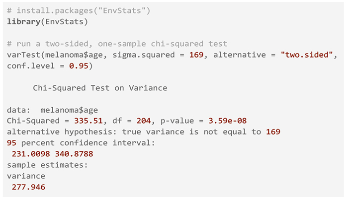
The sample variance of age is 277.95 and the two-sided, one-sample chi-squared test for variance computes a p-value of 3.59e-8. Since the p-value is less than the significance level of α=0.05, we reject the null hypothesis and conclude that the variance in age is different than 169. This is corroborated by the 95% confidence interval; it suggests that we are 95% confident that the true population variance of age is between 231.01 and 340.88, which does not include the hypothesized value of 169.
4. Multivariate Hypothesis Testing
So far, we have covered univariate hypothesis testing. This section focuses on tests for multiple population parameters.
The F-test is used to test if the variance of two groups are equal and uses the F-statistic. This test is particularly useful for checking the equal variance assumption for a two-sample t-test. The assumptions for the F-test are the following4:
Below we illustrate an F-test comparing tumor thickness variance between males and females. Using a two-tailed alternative hypothesis, we test if the tumor thickness population variance of males (σM2) is different from females (σF2). We define the null and alternative hypotheses as:
H0: σM2 = σF2. The population tumor thickness variance is the same for males and females.
HA: σM2 ≠ σF2. The population tumor thickness variance is different between males and females.
We then run a two-sided F-test with the R code shown below. By default, the var.test function computes a two-tailed hypothesis test and estimates the 95% confidence interval for the population mean. The arguments x (continuous variable ~ categorical variable), and data (name of dataset) are used to specify the dataset variables to test. We also have the option to specify a one or two-sided alternative hypothesis and the confidence level.
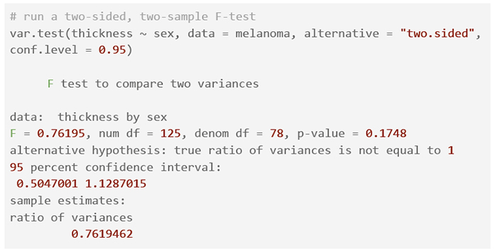
The ratio of the female/male age variance is 0.76 and the two-sided, two-sample F-test computes a p-value of 0.1748. Since the p-value is greater than than the significance level of α=0.05, we fail to reject the null hypothesis and cannot conclude that the tumor thickness variance is different between males and females. This is corroborated by the 95% confidence interval since it includes a ratio of 1. The confidence interval suggests that we are 95% confident that the true ratio of male vs. female age variance of our population is between 0.50 and 1.13.
4.2 Linear Relationship Between Two Numerical Variables
The Pearson’s correlation coefficient is used to test if two numeric variables are linearly associated and, if they are, the strength of their association. The correlation coefficient value is always between -1 and 1, where negative values indicate an inverse relationship and positive values indicate a positive relationship. By rule of thumb, absolute values between 0 to 0.39 indicate a weak relationship, 0.4 to 0.69 indicate a moderately strong relationship, and 0.7 to 1 indicate a strong relationship9. Pearson’s correlation coefficient only applies to linear relationships and cannot capture non-linearity.
The assumptions for the Pearson’s correlation test are the following9:
Below we illustrate computing the Pearson’s correlation coefficient between tumor thickness and age. Using a two-tailed alternative hypothesis, we test if the correlation coefficient (ρ) is significantly different from 0. We define the null and alternative hypotheses as:
H0: ρ = 0. The correlation between tumor thickness and age is 0.
HA: ρ ≠ 0. The correlation between tumor thickness and age is not 0.
We then run a correlation test with the code shown below. By default, the cor.test function computes a two-tailed hypothesis test and estimates the 95% confidence interval for Pearson’s correlation coefficient. The arguments x and y are used to specify the two variables to test. We also have the option to specify a one or two-sided alternative hypothesis and the confidence level.
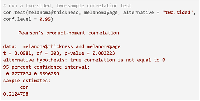
The output of the correlation test computes a Pearson’s correlation coefficient of 0.21 and a p-value of 0.0022. Since the p-value is less than than the significance level of α=0.05, we reject the null hypothesis and conclude that the relationship between tumor thickness and age is statistically significant. The 95% confidence interval suggests that we are 95% confident that the true correlation coefficient is between 0.08 and 0.34. Note that the lower bound is close to 0, indicating that the linear relationship is weak.
4.3 Population Means of Two Groupings
To test if the mean of a variable of interest in one group is different than that of another group, we use a two-sample t-test.
The assumptions for a two-sample t-test are7:
Below we illustrate a two-sided, two-sample t-test comparing tumor thickness between males and females, assuming equal variances between the groupings. Using a two-tailed alternative hypothesis, we test if the tumor thickness population mean of males (μm) is different from females (μf). We define the null and alternative hypotheses as:
Ho: μm = μf. The population mean tumor thickness is the same between males and females.
Ha: μm ≠ μf. The population mean tumor thickness is different between males and females.
We then run a two-sided, two-sample t-test with the code shown below. By default, the t.test function computes a two-tailed hypothesis test and estimates the 95% confidence interval for the population mean difference. The arguments x (continuous variable ~ categorical variable), and data (name of dataset) are used to specify the dataset variables to test. We also have the option to specify a one or two-sided alternative hypothesis and the confidence level. In a two-sample t-test, it is necessary to specify whether the variances of the groupings are equal or unequal. The default value is var.equal = FALSE. In Section 4.1 we were not able to conclude that the tumor thickness variance is different between males and females. Hence, we set var.equal = TRUE to compute a pooled variance that estimates the common variance between the two groupings.
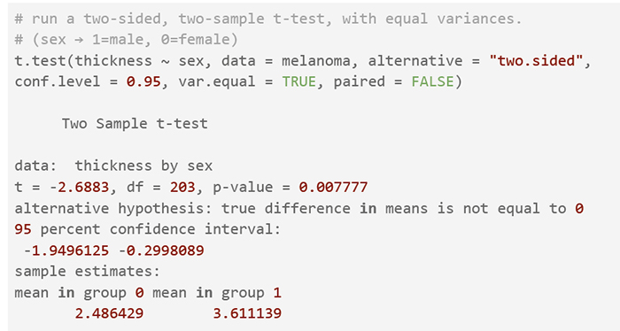
The sample mean of tumor thickness is 2.49 millimeters among females and 3.61 millimeters among males, rendering a sample difference of -1.12. The output of the two-sided t-test assuming equal variances computes a p-value of 0.0078. Since the p-value is less than the significance level of α=0.05, we reject the null hypothesis and conclude that there exists a difference in tumor thickness between males and females. This is corroborated by the 95% confidence interval; it suggests that we are 95% confident that the true mean difference is between -1.95 and -0.30, which does not include the null hypothesized difference of zero.
The two-sample t-test described above is based on the assumption that the two groupings are unrelated (independent). When assessing relationships between two groups, we hope that they are comparable in all their characteristics except for the one we are interested in. Because this is often not guaranteed, an option is to pair each individual in one group with an individual in the other group to ensure that the paired individuals are similar. The paired t-test takes into account the pairing of observations and, therefore, does not assume independence between the groups10. This test is also applied when we are comparing the same group of people before or after an intervention, meaning that the two groups include the same participants under different conditions. Using the difference between the paired observations, the hypothesis testing problem reduces to a single sample t-test problem. A paired t-test can be computed setting the paired argument equal to TRUE in the t.test function in R.
4.4 Population Proportions of Two or More Groupings
To test the association between two categorical variables, each with two or more groupings, we use the chi-squared (X2) test of independence. The chi-squared test statistic is computed by building a contingency table that compares the actual versus the expected counts of each combination of the groupings. If both variables are independent, the relative frequencies of the groupings of the first categorical variable are expected to be similar across the groupings of the second categorical variable.
The assumptions for the chi-squared test of independence test are10:
Below we illustrate a chi-squared test comparing tumor thickness between males and females, assuming equal variances between the groupings. Using a two-tailed alternative hypothesis, we test if the proportion of ulcer indication in males (pm) is different than in females (pm). We define the null and alternative hypotheses as:
Ho: pm = pf. The proportion of ulcer indication is the same between males and females.
Ha: pm ≠ pf. The proportion of ulcer indication is different between males and females.
We then run a two-sided, two-sample chi-squared test with the code shown below. First, we use the table function in R to verify the assumption of at least 5 observations per group combination. The chisq.test function uses as input the frequency table created in the first step of the code.
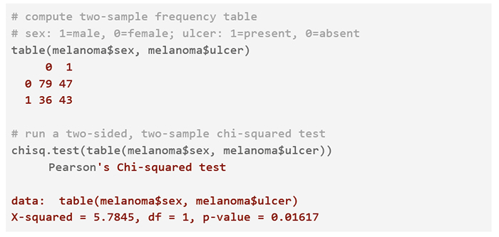
The output of the two-sided, two-sample chi-squared test for ulcer indication vs. sex computes a p-value of 0.0162. Since the p-value is less than the significance level of α=0.05, we reject the null hypothesis and conclude that there exists a difference in the proportion of ulcer indication between males and females.
4.5 Population Means of Two or More Groupings
The t-test can be used for tests involving one or two groups. Using a t-test for three groups or more would involve a comparison of group 1 vs. group 2, group 1 vs. group 3, and group 2 vs. group 3, individually. The number of t-tests would increase exponentially with more groups. The one-way ANOVA test is a solution. The test determines if any group is different from the rest of the groups. ANOVA stands for Analysis of Variance because it compares the variance of any group against the overall variance between groups. The test statistic is the F-value.
The assumptions for a one-way ANOVA test are10:
Here we illustrate an ANOVA test comparing age within each survival status (1 = died from melanoma, 2 = still alive, 3 = died from causes other than melanoma). We test if there exists a mean age difference between the three status groups. Let µ1, µ2 , and µ3 represent the population mean age for status groups 1, 2, and 3, respectively. We define the null and alternative hypotheses as:
H0: µ1 = µ2 = µ3. The mean age is the same between all three status groups.
HA: µ1 ≠ µ2 or µ1 ≠ µ3 or µ2 ≠ µ3. The mean age of at least one status group is different from the age of the other status groups.
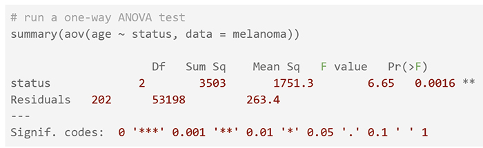
The one-way ANOVA test is run in R with the aov function. We use the summary function to obtain a detailed output that includes the p-value. In the example we see an F-value of 6.65 and a p-value of 0.0016. Since the p-value is less than the significance level of α=0.05, we can conclude that there is a difference in mean age between the status groups.
Interpretations of hypothesis testing methods are often reduced to whether the p-value passes a certain threshold to claim statistical significance. However, as the ASA's statement on p-values asserts, “Practices that reduce data analysis or scientific inference to mechanical “bright-line” rules (such as “p < 0.05”) for justifying scientific claims or conclusions can lead to erroneous beliefs and poor decision making”11. Indeed, statistical assertions based on such concepts distort the scientific process by failing to incorporate into the analysis the model assumptions, the overall statistical method, and all the results relating to the research question. Data analysis should not end with the calculation of a p-value when other approaches are appropriate and feasible11. Rather than focusing on individual findings, authors must disclose all the statistical analyses they run, even if the results are not statistically significant.
Greenland et al. assert that the estimation of the size of an association and the uncertainty around the estimate could be more relevant for scientific inference than arbitrary classifications on significance6. Note that a p-value does not measure the size of an association or the importance of a result11. Smaller p-values do not necessarily imply larger or more important effects and larger p-values do not necessarily imply unimportant associations or lack of effects. P-values are sensitive to the sample size. Hence, a large sample size may produce small p-values even when associations are not meaningful and vice versa. Additionally, given that p-values are based on the study assumptions, any violation of the protocol would invalidate any conclusion of statistical significance6. Therefore, p-values without context or other evidence are not enough.
Given the limitations and widespread misinterpretations of p-values, a few scientific journals now discourage their use and a few statisticians recommend their abandonment. Some alternatives to p-values that have been previously mentioned in literature are methods like confidence intervals, Bayes factors, and practical significance. Nevertheless, as statisticians Gelman and Carlin state, these replacements are also faulty because they still try to “get near-certainty out of noisy estimates” by using a summary statistic or threshold5. They suggest the use of larger, more informative models as alternatives to hypothesis testing and p-values. Such models require Bayesian inference or non-Bayesian regularization techniques such as Lasso to estimate continuous parameters. Although these alternative methods pose a great challenge to statistical pedagogy given their complexity, they highlight the “need to move toward a greater acceptance of uncertainty and embracing of variation”5. Evidence-based data analysis should be the ultimate goal. Education that reinforces good statistical practice is vital to improve the quality of published research.
Conflict of Interest
The authors declare that they have no conflict of interest.
Funding Sources
The study did not require funding sources.
Author Contributions
IZ: Analysis interpretation, R analysis, figures, and code.
IZ, MCV: Write-up
MCV: Content outline and edits.
All the authors read and approved the final version of the manuscript.
CITAR ESTE ARTÍCULO:
Zhao I, Velasco MC. Hypothesis Testing. Metro Ciencia [Internet]. 30 de marzo de 2022; 30(1):83-96. https://doi.org/10.47464/MetroCiencia/vol30/1/2022/83-96
MetroCiencia VOL. 30 Nº 1 (2022)